Python notebooks
Notebooks combine Python, SQL and Markdown cells in one document. They are standard Jupyter .ipynb files stored in the notebooks folder of your workspace, so you can open them in other tools too. Open the list with Ctrl+4.
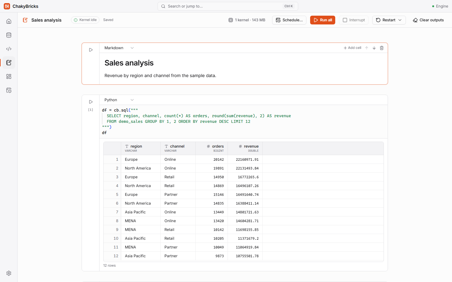
The notebook list
Notebooks lists your notebooks, with options to create, Rename… (renames the .ipynb file; jobs that use it follow along) and Delete…. On a table's page in the Catalog, Open in notebook creates a notebook with starter cells for that table.
Working in a notebook
- Cells are Python, SQL or Markdown; switch a cell's type with the menu at its top left. Hover between cells, or use the buttons at the bottom, to add + Code, + SQL or + Markdown; each cell's toolbar can add a cell above or below, move it up or down, and delete it.
- Run a cell with Shift+Enter (run and move to the next cell), Ctrl+Enter (run and stay) or Alt+Enter (run and insert a new cell below), or with the play button.
- The toolbar has Run all, Interrupt, Restart (restart the kernel, restart and clear outputs, or restart and run all), Clear outputs and Schedule… (see Jobs).
- Each cell shows its execution counter and how long it took. Queued cells run in order; as in Jupyter, an error stops the rest of the queue.
- Notebooks save automatically a moment after you stop typing.
- The kernel starts when you open a notebook; a badge shows its state. The first notebook in a workspace takes a few seconds longer while the workspace's Python environment is created. A small indicator in the toolbar shows how many kernels are running and their memory; Settings lists them and lets you shut them down.
Outputs
- Tables. DataFrames (Polars, pandas) and Arrow tables are shown in the same grid as the SQL editor: the first 1,000 rows plus the total row count.
- Charts. matplotlib figures show inline; Plotly figures are interactive.
- Text, errors and more.
printoutput streams as it happens, tracebacks are formatted, and images, HTML, SVG and Markdown outputs render.
SQL cells
A cell of type SQL (or any cell that starts with %%sql) runs SQL against your tables and shows the result as a table:
The optional name after %%sql stores the result in a Python variable (here sales_by_region, a Polars DataFrame) for later cells. SQL cells run the same statements as the SQL editor, including CREATE TABLE … AS SELECT and the other writes. In a SQL cell, errors are short and show only the SQL message.
cb reference
cb is preloaded in every notebook; there is nothing to import. It works on the same tables as the SQL editor.
cb.sql(query)
Runs SQL over your catalog tables and returns the result of the last statement as a Polars DataFrame. Use .to_pandas() on it for pandas.
It accepts several statements separated by semicolons and the same writes as the SQL editor (CREATE [OR REPLACE] TABLE … AS SELECT, INSERT INTO … SELECT|VALUES, DROP TABLE, ALTER TABLE … RENAME TO). A write prints its message and, if it was the last statement, cb.sql returns None.
cb.table(name, version=None)
Returns a lazy Polars frame (LazyFrame) over a table. Nothing is loaded until you .collect(), and Polars pushes filters and column selections down to the data, so this is the way to work with tables that are bigger than memory.
lazy = cb.table("main.sales")
top = lazy.filter(pl.col("amount") > 100).group_by("region").agg(pl.col("amount").sum()).collect()

old = cb.table("sales", version=3)   # time travel: the table as of Delta version 3
name is schema.table, or just table for the main schema. Versions are listed on the table's History tab.
cb.save(df, name, mode="overwrite", partition_by=None)
Writes a DataFrame to a Delta table and registers it in the catalog, so it shows up in the Catalog, the SQL editor and dashboards straight away.
df: a Polars DataFrame or LazyFrame, a pandas DataFrame or Series, or an Arrow table.name:schema.table, or justtableformain. The schema is created if it does not exist.mode:"overwrite"(default) replaces the table;"append"adds rows, and creates the table if it does not exist yet.partition_by: optional column to partition a new or replaced table by (ignored when appending to an existing table).
Column names are cleaned so they work unquoted in SQL and Python (the same rules as imports); when a name changes, cb.save prints a note. It returns a dictionary with the table, rows, version and columns of the result.
cb.tables()
The catalog as a Polars DataFrame, one row per table, with the columns schema, table, rows, size_bytes, version and updated_at.
Packages, memory and the environment
- Included packages are listed under Settings and Python packages. Install more with
%pip install name;!shell commands run in the same environment. - Each notebook's query engine may use 50% of the memory limit by default (configurable under Notebook kernel memory). Polars and pandas use ordinary process memory in addition, so for very large tables prefer
cb.sqlaggregations andcb.tablelazy frames over loading everything with.to_pandas(). - Kernels stop when you close ChakyBricks. Notebook jobs run in their own private kernel and never touch the notebook file; see Jobs.